Introduction
At work, we were implementing this new feature that would allow our users see how a certain dataset was changing with time. To put simply, it was an innocent line graph. This was a fairly simple task. All we had to do was fetch the data points for the graph and plot them using D3 on the page.
The problem grew a bit more complex when the dataset started lacking consistency. When we tried to use our innocent way of plotting the graph, things escalated. Real quick.
The Problem
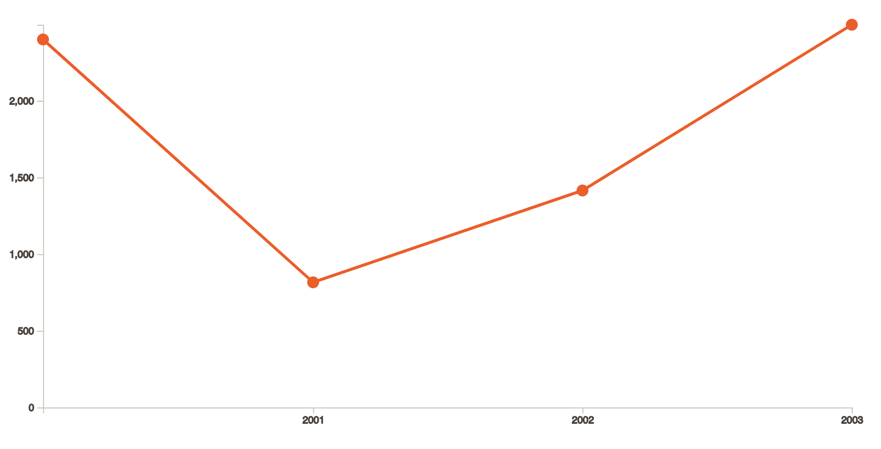
For a data set for the years 2000 - 2003, values [2400, 816, 1415, 2496] would generate a graph like above.
Our problem soon came as edge cases for when there would be missing data in the list as we integrated more and nore datasets in our db. Soon, our graphs would go either completely off the charts or would stop drawing different parts of the line, or worse, parse undefined or null as 0
To give you an example, here, the value for 2001 is set to null and the graph renders this value as 0.0
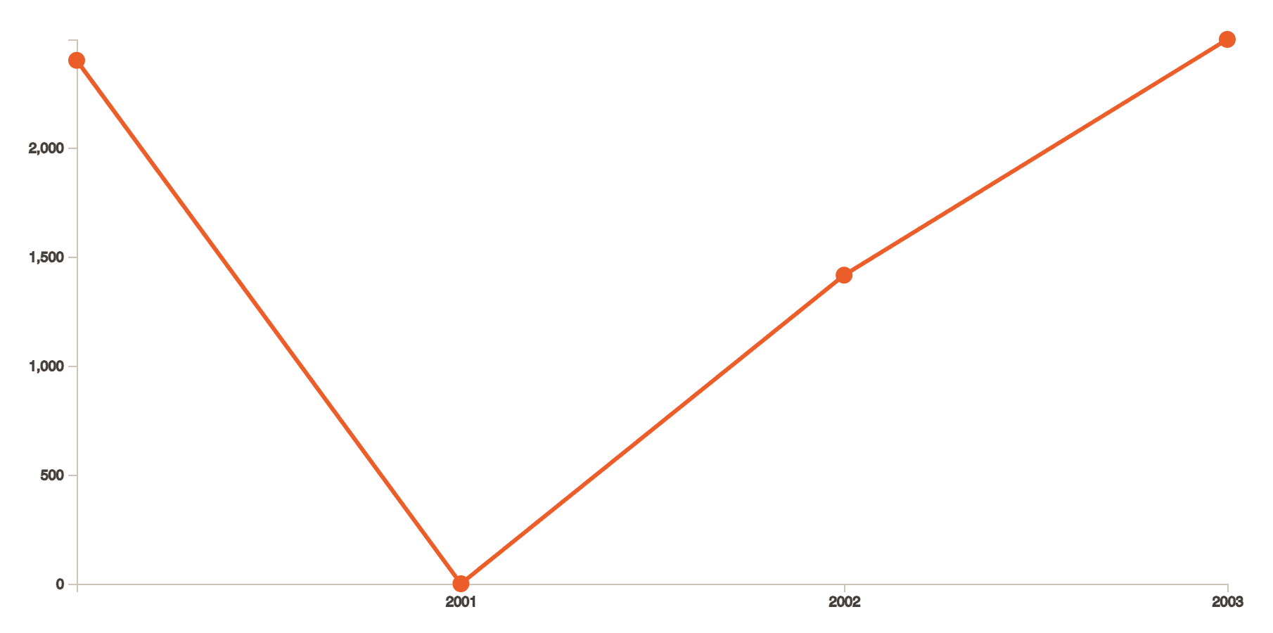
This became a huge problem since according to the data, it is supremely misleading. The value must be around 816. Imagine if this was a case if you were seeing the trend in currencies. Worse, if we were comparing 2 currencies.
We never saw this coming.
When Jerry, our UX Lead, saw this, he came to decision that it's better to show approximated values on the graph so that our users are not mislead and use grey to show to demarcate actual from approximated ones.
UX wise, this was a nifty trick. Programming wise, I had to go back to my college days to find a way.
The Math
The inter-webs was filled with examples on how people used the d3-interpolate library function to accomplish something similar. But interpolation doesn't do approximations.
Interpolation vs Regression
Interpolation is a way to find a line 𝐹(𝑥) such that for all values of 𝑥, there is an exact 𝑦. Regression is a way to find a line 𝐹(𝑥) such that when 𝐹(𝑥) is the closest to all values of 𝑥 at once.
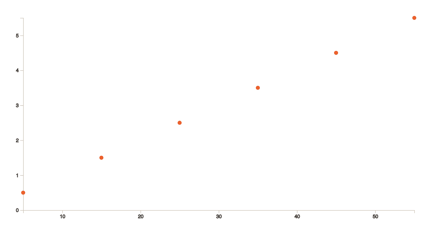
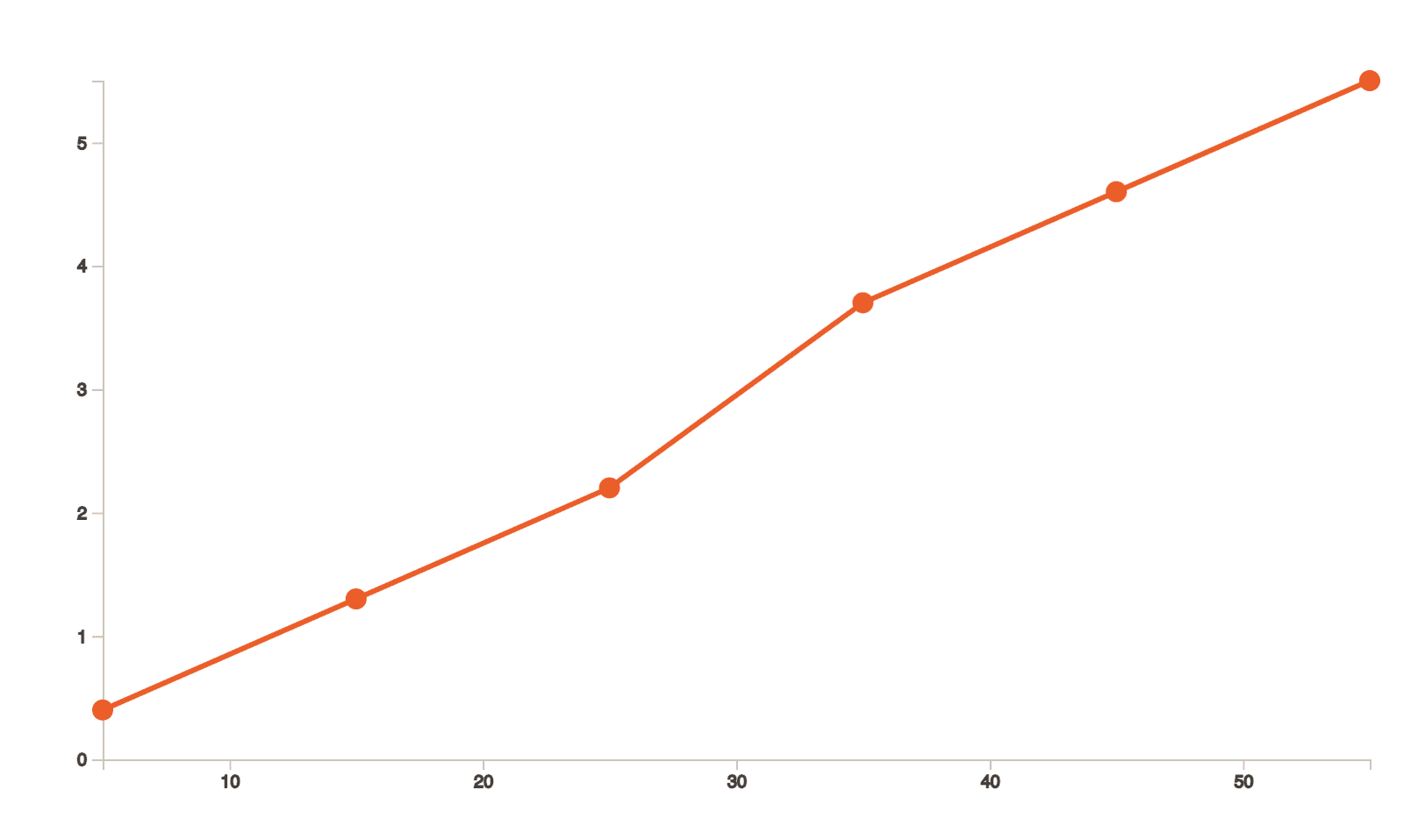
Take a look at the above line graph. For simpler cases, we probably do interpolation without even realizing it. For example, by looking at this chart above, if we were to find the value of 𝐹(𝑥) (or in other words 𝑦) when 𝑥 is 35, our brain would probably draw conclusions in seconds because the human brain understands visuals better.
Our brain would first try to imagine a line passing exactly through all the dots and then come to a conclusion of 3.5. The process of finding this line which passes through all these points is interpolation. We see best through visuals.
But what if the dots look like the following image and we want to estimate the value of 𝑦 when the value of 𝑥 is 25?
By looking at it, It could very well be any value between 2.2 or 2.5. Imagine if this dataset was about saving the cost of a dying organization. Imagine if the scales and stakes would go up and our guestimation was dwindling between 22 and 25 million USD.
Linear Regression
By looking at this graph, we are trying to find a similar line like we did in while interpolating. But we do not want it to pass exactly through the points. In fact, it should be as close as possible to all the points.
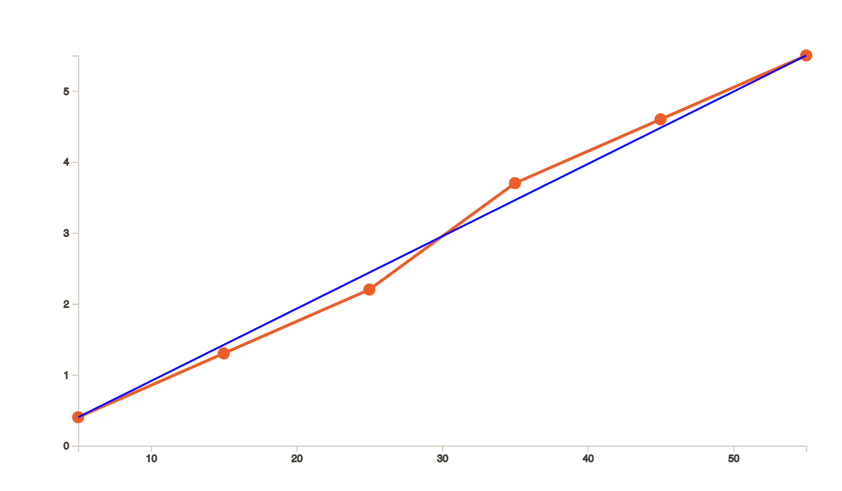
One way to do this is if we would start drawing the smallest squares from each dot so that if there is a line which touches the other end of the square, it is straight. This method is called the least squares method.
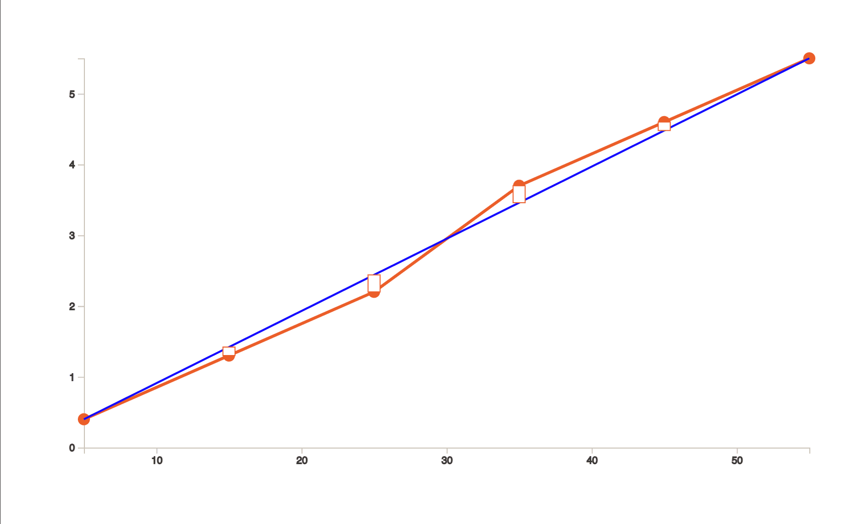
Now, if we were to estimate the value of 𝑦 when the value of 𝑥 is 25, or in other words, if we were to estimate 𝐹(25), we get to a conclusion that it should be 2.39.
I needed the computer to do this. Find the value of 𝑦 when the second number in the dataset was null. Programmatically.
The Code
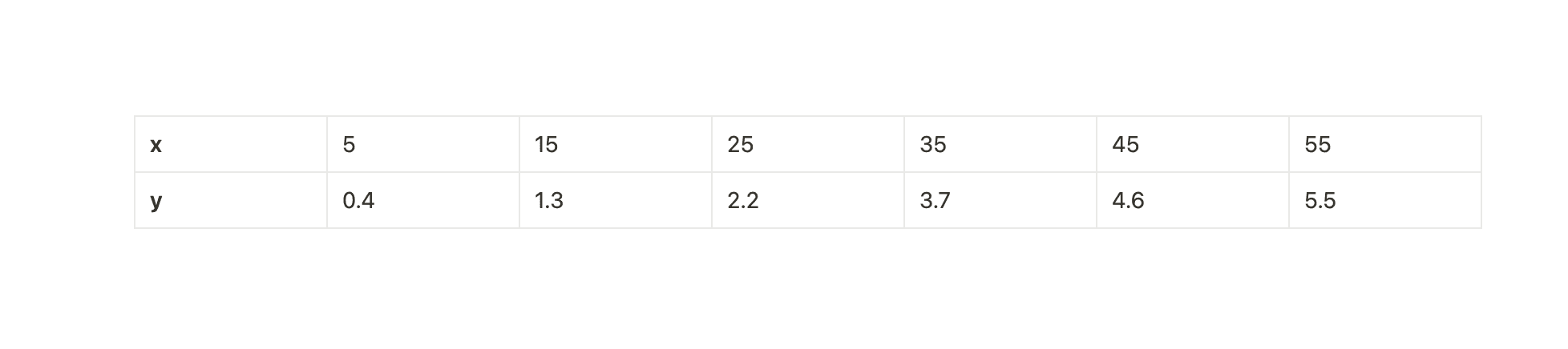
Our objective is to make the function of this line. Let's code along. We know that the a straight line follows the equation y = mx + c. Where y is our function, m is the slope or gradient of the line with respect to the webpage's bottom edge (horizontal axis) and x is what we need to solve for. Here's the dataset that built the scatterplot above.
The expression for finding the slope m is
(N Σ(xy) − Σx Σy)/ (N Σ(x sq.) − (Σx) sq)where N is the number of datapoints. Which means our function will also need all the datapoints to calculate the sum of all x square, xy, x, and y
m = (N Σ(xy) − Σx Σy)/ (N Σ(x sq.) − (Σx) sq)
c = (Σy − m Σx)/N
Conclusion
Of course, we were dealing with a [time, value] pairs instead of [value,value] pairs but our predictor function was similar. This use case was also solved quickly because the conditions to solve the problem met the criteria to use this technique.
Linear Regression should only be used when the data value pairs are somehow related. There are also outliers and residual plots we need to be aware of. This is where things start going supremely.